11.8. Deploying GeoMesa Spark with Jupyter Notebook¶

Jupyter Notebook is a web-based application for creating interactive documents containing runnable code, visualizations, and text. Via the Apache Toree kernel, Jupyter can be used for preparing spatio-temporal analyses in Scala and submitting them in Spark. The guide below describes how to configure Jupyter with Spark 3.5 and GeoMesa.

Note

GeoMesa support for PySpark provides access to GeoMesa Accumulo data stores through the Spark Python API using Jupyter’s built in Python kernel. See GeoMesa PySpark.

11.8.1. Prerequisites¶

Spark 3.5 should be installed, and the environment variable SPARK_HOME should be set.

Python 2.7 or 3.x should be installed, and it is recommended that Jupyter and Toree are installed inside a Python virtualenv or inside a conda environment.

11.8.2. Installing Jupyter¶

Jupyter may be installed via pip (for Python 2.7) or pip3 (for Python 3.x):

$ pip install --upgrade jupyter

or

$ pip3 install --upgrade jupyter

11.8.3. Installing the Toree Kernel¶

$ pip install --upgrade toree

or

$ pip3 install --upgrade toree

11.8.4. Configure Toree and GeoMesa¶

If you have the GeoMesa Accumulo distribution installed at GEOMESA_ACCUMULO_HOME as described in Setting up the Accumulo Command Line Tools, you can run the following example script to configure Toree with GeoMesa:

Note

Ensure that the Scala version you use matches the Scala version of your Spark version.

$ export TAG="5.1.0"
$ export VERSION="2.12-${TAG}" # note: 2.12 is the Scala build version

#!/bin/sh

# bundled GeoMesa Accumulo Spark and Spark SQL runtime JAR
# (contains geomesa-accumulo-spark, geomesa-spark-core, geomesa-spark-sql, and dependencies)
jars="file://$GEOMESA_ACCUMULO_HOME/dist/spark/geomesa-accumulo-spark-runtime-accumulo21_$VERSION.jar"

# uncomment to use the converter RDD provider
#jars="$jars,file://$GEOMESA_ACCUMULO_HOME/lib/geomesa-spark-converter_$VERSION.jar"

# uncomment to work with shapefiles (requires $GEOMESA_ACCUMULO_HOME/bin/install-shapefile-dependencies.sh)
#jars="$jars,file://$GEOMESA_ACCUMULO_HOME/lib/jai_codec-1.1.3.jar"
#jars="$jars,file://$GEOMESA_ACCUMULO_HOME/lib/jai_core-1.1.3.jar"
#jars="$jars,file;//$GEOMESA_ACCUMULO_HOME/lib/jai_imageio-1.1.jar"

jupyter toree install \
    --replace \
    --user \
    --kernel_name "GeoMesa Spark $VERSION" \
    --spark_home=${SPARK_HOME} \
    --spark_opts="--master yarn --jars $jars"

Note

The JARs specified will be in the respective target directory of each module of the source distribution if you built GeoMesa from source.

Note

You may wish to change --spark_opts to specify the number and configuration of your executors; otherwise the values in $SPARK_HOME/conf/spark-defaults.conf or $SPARK_OPTS will be used.

You may also consider adding geomesa-tools_${VERSION}-data.jar to include prepackaged converters for publicly available data sources (as described in Prepackaged Converter Definitions), geomesa-spark-jupyter-leaflet_${VERSION}.jar to include an interface for the Leaflet spatial visualization library (see Leaflet for Visualization, below).

11.8.5. Running Jupyter¶

For public notebooks, you should configure Jupyter to use a password and bind to a public IP address (by default, Jupyter will only accept connections from localhost). To run Jupyter with the GeoMesa Spark kernel:

$ jupyter notebook

Note

Long-lived processes should probably be hosted in screen, systemd, or supervisord.

Your notebook server should launch and be accessible at http://localhost:8888/ (or the address and port you bound the server to), potentially requiring an access token which will be shown in the server output.

Note

All Spark code will be submitted as the user account running the Jupyter server. You may wish to look at JupyterLab for a multi-user Jupyter server.

11.8.6. Leaflet for Visualization¶

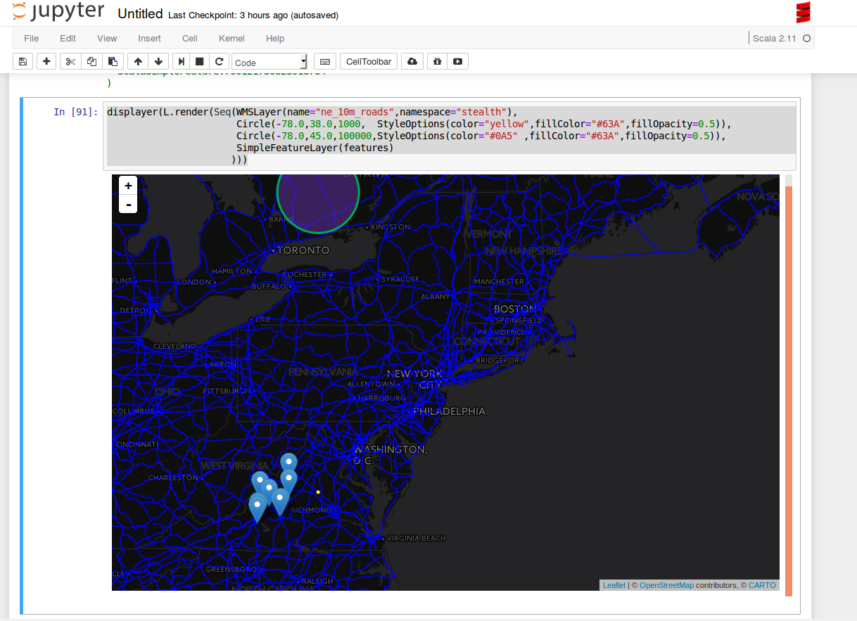
The following sample notebook shows how you can use Leaflet for data visualization:

classpath.addRepository("https://repo1.maven.org/maven2")
classpath.addRepository("https://repo.osgeo.org/repository/release")
classpath.addRepository("file:///home/username/.m2/repository")
classpath.add("org.locationtech.geomesa" % "geomesa-accumulo-datastore_2.12" % "4.0.0")
classpath.add("org.locationtech.geomesa" % "geomesa-spark-jupyter-leaflet_2.12" % "4.0.0")
classpath.add("org.locationtech.jts" % "jts-core" % "1.19.0")
classpath.add("org.apache.accumulo" % "accumulo-core" % "2.0.1")

import org.locationtech.geomesa.accumulo.data.AccumuloDataStoreParams._
import org.locationtech.geomesa.jupyter._
import org.locationtech.geomesa.utils.geotools.Conversions._
import scala.collection.JavaConverters._

implicit val displayer: String => Unit = display.html(_)

val params = Map(
        ZookeepersParam.key   -> "ZOOKEEPERS",
        InstanceNameParam.key -> "INSTANCE",
        UserParam.key         -> "USER_NAME",
        PasswordParam.key     -> "USER_PASS",
        CatalogParam.key      -> "CATALOG")

val ds = org.geotools.api.data.DataStoreFinder.getDataStore(params.asJava)
val ff = org.geotools.factory.CommonFactoryFinder.getFilterFactory
val fs = ds.getFeatureSource("twitter")

val filt = ff.and(
    ff.between(ff.property("dtg"), ff.literal("2016-01-01"), ff.literal("2016-05-01")),
    ff.bbox("geom", -80, 37, -75, 40, "EPSG:4326"))
val features = fs.getFeatures(filt).features.asScala.take(10).toList

displayer(L.render(Seq(WMSLayer(name="ne_10m_roads",namespace="NAMESPACE"),
                       Circle(-78.0,38.0,1000,  StyleOptions(color="yellow",fillColor="#63A",fillOpacity=0.5)),
                       Circle(-78.0,45.0,100000,StyleOptions(color="#0A5" ,fillColor="#63A",fillOpacity=0.5)),
                       SimpleFeatureLayer(features)
                      )))

11.8.6.1. Adding Layers to a Map and Displaying in the Notebook¶

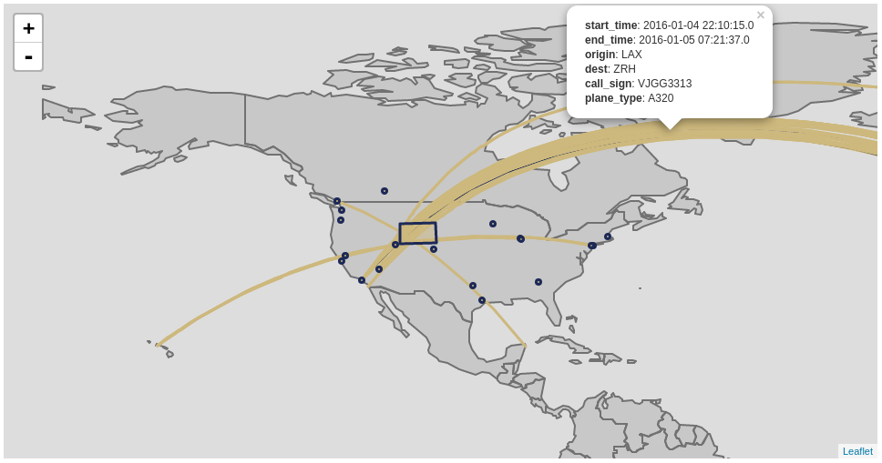
The following snippet is an example of rendering dataframes in Leaflet in a Jupyter notebook:

implicit val displayer: String => Unit = { s => kernel.display.content("text/html", s) }

val function = """
function(feature) {
  switch (feature.properties.plane_type) {
    case "A388": return {color: "#1c2957"}
    default: return {color: "#cdb87d"}
  }
}
"""

val sftLayer = time { L.DataFrameLayerNonPoint(flights_over_state, "__fid__", L.StyleOptionFunction(function)) }
val apLayer = time { L.DataFrameLayerPoint(flyovers, "origin", L.StyleOptions(color="#1c2957", fillColor="#cdb87d"), 2.5) }
val stLayer = time { L.DataFrameLayerNonPoint(queryOnStates, "ST", L.StyleOptions(color="#1c2957", fillColor="#cdb87d", fillOpacity= 0.45)) }
displayer(L.render(Seq[L.GeoRenderable](sftLayer,stLayer,apLayer),zoom = 1, path = "path/to/files"))

11.8.6.2. StyleOptionFunction¶

This case class allows you to specify a Javascript function to perform styling. The anonymous function that you will pass takes a feature as an argument and returns a Javascript style object. An example of styling based on a specific property value is provided below:

function(feature) {
  switch(feature.properties.someProp) {
    case "someValue": return { color: "#ff0000" }
    default         : return { color: "#0000ff" }
  }
}

The following table provides options that might be of interest:

Option	Type	Description
color	String	Stroke color
weight	Number	Stroke width in pixels
opacity	Number	Stroke opacity
fillColor	String	Fill color
fillOpacity	Number	Fill opacity

Note: Options are comma-separated (i.e. { color: "#ff0000", fillColor: "#0000ff" })