GeoMesa HBase Quick Start
This tutorial is the fastest and easiest way to get started with GeoMesa using HBase. It is a good stepping-stone on the path to the other tutorials, that present increasingly involved examples of how to use GeoMesa.
About this Tutorial
In the spirit of keeping things simple, the code in this tutorial only does a few small things:
Establishes a new (static) SimpleFeatureType
Prepares the HBase tables to store this type of data
Creates a few thousand example SimpleFeatures
Writes these SimpleFeatures to HBase
Queries for a given geographic rectangle, time range, and attribute filter, writing out the entries in the result set
Uses GeoServer to visualize the data (optional)
Prerequisites
Before you begin, you must have the following installed and configured:
Java JDK 1.8
Apache Maven 3.5.2 or later
a GitHub client
an HBase 1.4.x or 2.2.x instance
the GeoMesa HBase distributed runtime installed for your HBase instance (see below)
If you do not have an existing HBase instance, you can easily set one up as detailed next.
Setting up HBase in standalone mode (optional)
(Skip this section if you have an existing HBase 1.4.x or 2.2.x installation.)
Download the HBase 1.4.13 binary distribution from https://hbase.apache.org/downloads.html
Follow the chapter in the HBase Manual for running a standalone instance of HBase (https://hbase.apache.org/book.html#quickstart). Note that this will use the local filesystem instead of HDFS, and will spin up its own instances of HBase and Zookeeper.
Installing the GeoMesa Distributed Runtime
Follow the instructions under Installing the GeoMesa Distributed Runtime JAR and Register the Coprocessors to install GeoMesa in your HBase instance.
Download and Build the Tutorial
Pick a reasonable directory on your machine, and run:
$ git clone https://github.com/geomesa/geomesa-tutorials.git
$ cd geomesa-tutorials
Warning
Make sure that you download or checkout the version of the tutorials project that corresponds to your GeoMesa version. See About Tutorial Versions for more details.
To ensure that the quick start works with your environment, modify the pom.xml
to set the appropriate versions for HBase, Hadoop, etc.
For ease of use, the project builds a bundled artifact that contains all the required dependencies in a single JAR. To build, run:
$ mvn clean install -pl geomesa-tutorials-hbase/geomesa-tutorials-hbase-quickstart -am
Running the Tutorial
On the command line, run:
$ java -cp geomesa-tutorials-hbase/geomesa-tutorials-hbase-quickstart/target/geomesa-tutorials-hbase-quickstart-$VERSION.jar \
    org.geomesa.example.hbase.HBaseQuickStart \
    --hbase.zookeepers <zookeepers>           \
    --hbase.catalog <table>
where you provide the following arguments:
<zookeepers>the HBase Zookeeper quorum. If you installed HBase in stand-alone mode, this will belocalhost. Note that for most use cases, it is preferable to put thehbase-site.xmlfrom your cluster on the GeoMesa classpath instead of specifying Zookeepers.<table>the name of the destination table that will accept these test records. This table should either not exist or should be empty
Optionally, you can also specify that the quick start should delete its data upon completion. Use the
--cleanup flag when you run to enable this behavior.
Once run, you should see the following output:
Loading datastore

Creating schema: GLOBALEVENTID:String,Actor1Name:String,Actor1CountryCode:String,Actor2Name:String,Actor2CountryCode:String,EventCode:String,NumMentions:Integer,NumSources:Integer,NumArticles:Integer,ActionGeo_Type:Integer,ActionGeo_FullName:String,ActionGeo_CountryCode:String,dtg:Date,geom:Point:srid=4326

Generating test data

Writing test data
Wrote 2356 features

Running test queries
Running query BBOX(geom, -120.0,30.0,-75.0,55.0) AND dtg DURING 2017-12-31T00:00:00+00:00/2018-01-02T00:00:00+00:00
01 719027236=719027236|UNITED STATES|USA|INDUSTRY||012|1|1|1|3|Central Valley, California, United States|US|2018-01-01T00:00:00.000Z|POINT (-119.682 34.0186)
02 719027005=719027005|UNITED STATES|USA|||172|2|2|2|3|Long Beach, California, United States|US|2018-01-01T00:00:00.000Z|POINT (-118.189 33.767)
03 719026204=719026204|JUDGE||||0214|6|1|6|3|Los Angeles, California, United States|US|2018-01-01T00:00:00.000Z|POINT (-118.244 34.0522)
04 719025745=719025745|KING||||051|4|2|4|2|California, United States|US|2018-01-01T00:00:00.000Z|POINT (-119.746 36.17)
05 719026858=719026858|UNITED STATES|USA|||010|20|2|20|2|California, United States|US|2018-01-01T00:00:00.000Z|POINT (-119.746 36.17)
06 719026964=719026964|UNITED STATES|USA|||081|2|2|2|2|California, United States|US|2018-01-01T00:00:00.000Z|POINT (-119.746 36.17)
07 719026965=719026965|CALIFORNIA|USA|||081|8|1|8|2|California, United States|US|2018-01-01T00:00:00.000Z|POINT (-119.746 36.17)
08 719025635=719025635|PARIS|FRA|||010|2|1|2|3|Las Vegas, Nevada, United States|US|2018-01-01T00:00:00.000Z|POINT (-115.137 36.175)
09 719026918=719026918|UNITED STATES|USA|||042|20|5|20|3|Las Vegas, Nevada, United States|US|2018-01-01T00:00:00.000Z|POINT (-115.137 36.175)
10 719027141=719027141|ALABAMA|USA|JUDGE||172|8|1|8|2|Nevada, United States|US|2018-01-01T00:00:00.000Z|POINT (-117.122 38.4199)

Returned 669 total features

Running query BBOX(geom, -120.0,30.0,-75.0,55.0) AND dtg DURING 2017-12-31T00:00:00+00:00/2018-01-02T00:00:00+00:00
Returning attributes [GLOBALEVENTID, dtg, geom]
01 719027208=719027208|2018-01-01T00:00:00.000Z|POINT (-89.6812 32.7673)
02 719026313=719026313|2018-01-01T00:00:00.000Z|POINT (-84.388 33.749)
03 719026419=719026419|2018-01-01T00:00:00.000Z|POINT (-84.388 33.749)
04 719026316=719026316|2018-01-01T00:00:00.000Z|POINT (-83.6487 32.9866)
05 719027132=719027132|2018-01-01T00:00:00.000Z|POINT (-81.2793 33.4968)
06 719026819=719026819|2018-01-01T00:00:00.000Z|POINT (-81.9296 33.7896)
07 719026952=719026952|2018-01-01T00:00:00.000Z|POINT (-81.9296 33.7896)
08 719026881=719026881|2018-01-01T00:00:00.000Z|POINT (-82.0193 34.146)
09 719026909=719026909|2018-01-01T00:00:00.000Z|POINT (-82.0193 34.146)
10 719026951=719026951|2018-01-01T00:00:00.000Z|POINT (-82.0193 34.146)

Returned 669 total features

Running query EventCode = '051'
01 719024909=719024909|||MELBOURNE|AUS|051|10|1|10|4|Melbourne, Victoria, Australia|AS|2018-01-01T00:00:00.000Z|POINT (144.967 -37.8167)
02 719025178=719025178|AUSTRALIA|AUS|COMMUNITY||051|20|2|20|4|Sydney, New South Wales, Australia|AS|2018-01-01T00:00:00.000Z|POINT (151.217 -33.8833)
03 719025965=719025965|MIDWIFE||||051|10|1|10|4|Sydney, New South Wales, Australia|AS|2018-01-01T00:00:00.000Z|POINT (151.217 -33.8833)
04 719025509=719025509|COMMUNITY||AUSTRALIA|AUS|051|2|1|2|1|Australia|AS|2018-01-01T00:00:00.000Z|POINT (135 -25)
05 719025742=719025742|KING||||051|22|3|22|3|San Diego, California, United States|US|2018-01-01T00:00:00.000Z|POINT (-117.157 32.7153)
06 719025745=719025745|KING||||051|4|2|4|2|California, United States|US|2018-01-01T00:00:00.000Z|POINT (-119.746 36.17)
07 719025743=719025743|AUTHORITIES||||051|60|12|60|3|Wichita, Kansas, United States|US|2018-01-01T00:00:00.000Z|POINT (-97.3375 37.6922)
08 719027205=719027205|UNITED STATES|USA|SIOUX||051|4|1|4|3|Sioux City, Iowa, United States|US|2018-01-01T00:00:00.000Z|POINT (-96.4003 42.5)
09 719025111=719025111|||UNITED STATES|USA|051|2|1|2|3|Pickens County, South Carolina, United States|US|2018-01-01T00:00:00.000Z|POINT (-82.7165 34.9168)
10 719026938=719026938|PITTSBURGH|USA|||051|5|1|5|3|York County, Pennsylvania, United States|US|2018-01-01T00:00:00.000Z|POINT (-77 40.1254)

Returned 138 total features

Running query EventCode = '051' AND dtg DURING 2017-12-31T00:00:00+00:00/2018-01-02T00:00:00+00:00
Returning attributes [GLOBALEVENTID, dtg, geom]
01 719024909=719024909|2018-01-01T00:00:00.000Z|POINT (144.967 -37.8167)
02 719025178=719025178|2018-01-01T00:00:00.000Z|POINT (151.217 -33.8833)
03 719025965=719025965|2018-01-01T00:00:00.000Z|POINT (151.217 -33.8833)
04 719025509=719025509|2018-01-01T00:00:00.000Z|POINT (135 -25)
05 719025742=719025742|2018-01-01T00:00:00.000Z|POINT (-117.157 32.7153)
06 719025745=719025745|2018-01-01T00:00:00.000Z|POINT (-119.746 36.17)
07 719025743=719025743|2018-01-01T00:00:00.000Z|POINT (-97.3375 37.6922)
08 719027205=719027205|2018-01-01T00:00:00.000Z|POINT (-96.4003 42.5)
09 719025111=719025111|2018-01-01T00:00:00.000Z|POINT (-82.7165 34.9168)
10 719026938=719026938|2018-01-01T00:00:00.000Z|POINT (-77 40.1254)

Returned 138 total features

Cleaning up test data
Done
Looking at the Code
The source code is meant to be accessible for this tutorial. The main logic is contained in
the generic org.geomesa.example.quickstart.GeoMesaQuickStart in the geomesa-tutorials-common module,
which is datastore agnostic. Some relevant methods are:
createDataStoreget a datastore instance from the input configurationcreateSchemacreate the schema in the datastore, as a pre-requisite to writing datawriteFeaturesuse aFeatureWriterto write features to the datastorequeryFeaturesrun several queries against the datastorecleanupdelete the sample data and dispose of the datastore instance
The quickstart uses a small subset of GDELT data. Code for parsing the data into GeoTools SimpleFeatures is
contained in org.geomesa.example.data.GDELTData:
getSimpleFeatureTypecreates theSimpleFeatureTyperepresenting the datagetTestDataparses an embedded TSV file to createSimpleFeatureobjectsgetTestQueriesillustrates several different query types, using CQL (GeoTools’ Contextual Query Language)
Visualize Data (optional)
There are two options to visual the data ingested by this quick start. The easiest option is to use the
export command of the GeoMesa HBase tools distribution. For a more production ready example, you
can alternatively stand up a GeoServer and connect it to your HBase instance.
Visualize Data With Leaflet
Warning
To successfully run this command you must have a computer that is connected to the internet in order to access external Leaflet resources.
The export command is a part of the GeoMesa HBase command-line tools. In order to use the command,
ensure you have the command-line tools installed as described in Setting up the HBase Command Line Tools.
The export command provides the leaflet format which will export the features to a Leaflet map
that you can open in your web browser. To produce the map, run the following command from the GeoMesa
HBase tools distribution directory:
bin/geomesa-hbase export            \
    --output-format leaflet         \
    --feature-name gdelt-quickstart \
    --zookeepers <zookeepers>       \
    --catalog <table>
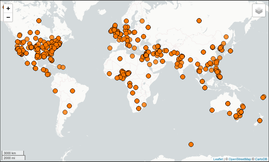
Where the connection parameters are the same you used above during the quickstart. To view the map simply open the url provided by the command in your web browser. If you click the menu in the upper right of the map you can enable and disable the heatmap and feature layers as well as the two provided base layers.

Visualizing quick-start data with Leaflet
Visualize Data With GeoServer
You can use GeoServer to access and visualize the data stored in GeoMesa. In order to use GeoServer, download and install version 2.17.3. Then follow the instructions in Installing GeoMesa HBase in GeoServer to enable GeoMesa.
Register the GeoMesa Store with GeoServer
Log into GeoServer using your user and password credentials. Click
“Stores” and “Add new Store”. Select the HBase (GeoMesa) vector data
source, and fill in the required parameters.
Basic store info:
workspacethis is dependent upon your GeoServer installationdata source namepick a sensible name, such asgeomesa_quick_startdescriptionthis is strictly decorative;GeoMesa quick start
Connection parameters:
these are the same parameter values that you supplied on the command line when you ran the tutorial; they describe how to connect to the HBase instance where your data reside
Click “Save”, and GeoServer will search your HBase table for any GeoMesa-managed feature types.
Publish the Layer
GeoServer should recognize the gdelt-quickstart feature type, and
should present that as a layer that can be published. Click on the
“Publish” link.
You will be taken to the “Edit Layer” screen. You will need to enter values for the data bounding boxes. In this case, you can click on the link to compute these values from the data.
Click on the “Save” button when you are done.
Take a Look
Click on the “Layer Preview” link in the left-hand gutter. If you don’t
see the quick-start layer on the first page of results, enter the name
of the layer you just created into the search box, and press
<Enter>.
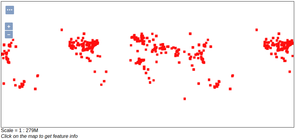
Once you see your layer, click on the “OpenLayers” link, which will open a new tab. You should see a collection of red dots similar to the following image:

Visualizing quick-start data with GeoServer
Tweaking the display
Here are just a few simple ways you can play with the visualization:
Click on one of the red points in the display, and GeoServer will report the detail records underneath the map area.
Shift-click to highlight a region within the map that you would like to zoom into.
Click on the “Toggle options toolbar” icon in the upper-left corner of the preview window. The right-hand side of the screen will include a “Filter” text box. Enter
EventCode = '051', and press on the “play” icon. The display will now show only those points matching your filter criterion. This is a CQL filter, which can be constructed in various ways to query your data. You can find more information about CQL from GeoServer’s CQL tutorial.
Generating Heatmaps
To try out server-side processing, you can install the Heatmap SLD from the Map-Reduce Ingest of GDELT tutorial.
After configuring the SLD, in the URL, change
styles=to bestyles=heatmap. Once you press<Enter>, the display will change to a density heat-map.
Note
For this to work, you will have to first install the WPS module for GeoServer as described in GeoServer Plugins.